Using tidymetadata-package with Luxembourdg Income Study data

Install the package with

devtools::install_github("muuankarski/tidymetadata")

Tidymetadata-package provides a technical backbone for tidy metadata logic to work with social survey data using tidyverse tools.

If not familiar with tidy data or tidyverse, please familiarise yourself with:

• Wickham, Hadley. 2014. ‘Tidy Data’. Journal of Statistical Software 59 (10). doi:10.18637/jss.v059.i10.
• R for Data Science: Tidy Data
• http://tidyverse.org/

Tidymetadata is not replacement for dedicated packages to work with survey data in general such as survey, but it complements them by providing a framework to deal with the labelled structure typical for social survey data. Such structure is not optimal to work with in R and tidyverse. Basically, tidymetadata provides functions to separate the data and metadata from labelled data.frame imported in R with haven and how to put it back together. This approach comes especially handy when building shiny-applications on top of such data. Try first running the shiny-app wrapped with the package with tidymetadata::runExample().

Download SPSS, Stata and SAS training data from Luxembourg Income Study

Survey datas are in most cases still disseminated in either SAS, SPSS or Stata formats with metadata included in variable and value labels. We first download the demo files freely available at from Luxembourg Income Study.

library(tidyverse)

if (!file.exists("./datasets/data.sav")){

  dir.create("./datasets")
  # SPSS-file

  download.file("http://www.lisdatacenter.org/wp-content/uploads/it04ip.sav", "./datasets/data.sav")
  # Stata-file

  download.file("http://www.lisdatacenter.org/wp-content/uploads/it04ip.dta", "./datasets/data.dta")
  # SAS-file

  download.file("http://www.lisdatacenter.org/wp-content/uploads/it04ip.sas7bdat", "./datasets/data.sas7bdat")

}

Package haven provides handy functions for reading in such formats

library(haven)
spss  <- read_sav("./datasets/data.sav")
stata <- read_dta("./datasets/data.dta")
sas   <- read_sas("./datasets/data.sas7bdat")

They all have the same number of cases and variables, and seem to share similar structure with variable labels and value labels as attributes. However, when applying str() function for all three datas we can spot that imported spss and stata files seem to have identical structure and somewhat richer than sas file has.

Create “tidy metadata”

Once we have datafiles in R, we use function tidymetadata::create_meta() to create tidy metadata. tidymetadata::create_meta() extracts the metadata information from variable attributes and creates a tidy data frame with columns:

• code for variable code
• name for variable name
• value for each value for each labelled variable
• label for each value label for each labelled variable
• class for wheter the variable in question is factor, numeric or character

As for rows, tidy metadata has a single row for a unique numeric or character type of variable. Such variables are not labelled ie. have no additional information within the object. As for factor variables, tidy metadata has one row per one value ie. factor level. For instance, two class gender variable would have two rows in tidy metadata, one for both values.

Lets apply the tidymetadata::create_meta()-function for each data:

library(tidymetadata)
meta_spss <- create_metadata(spss)
meta_stata <- create_metadata(stata)
meta_sas <- create_metadata(sas)

And, lets subset each data into variable sex and pile up the resulting rows:

meta_spss$type ="spss"

meta_stata$type ="stata"

meta_sas$type ="sas"



bind_rows(
          meta_spss[meta_spss$code == "sex",],
          meta_stata[meta_stata$code == "sex",],
          meta_sas[meta_sas$code == "sex",]
          ) %>% 


  knitr::kable()

code	name	label	value	class	type
sex	gender	[1]male	1	factor	spss
sex	gender	[2]female	2	factor	spss
sex	gender	[1]male	1	factor	stata
sex	gender	[2]female	2	factor	stata
sex	gender	NA	NA	numeric	sas

We can see that SPSS and Stata files produce identical metadatas for variable sex, but SAS file is lacking the value label information. For this reason we should work only using either Stata or SPSS files in this case, and for this particular vignette we will choose the SPSS file.

Stripping data from attributes

Once we have extracted the metadata information from the labelled data, we can strip off this information and leave only the bare data with numeric/character content in the variables using tidymetadata::strip_attributes() function with no attributes whatsoever.

Before stripping the attributes we get:

str(spss[,1:10])

## Classes 'tbl_df', 'tbl' and 'data.frame':    1358 obs. of  10 variables:
##  $ hid    : atomic  1 1 2 2 2 2 3 4 4 4 ...
##   ..- attr(*, "label")= chr "unique unit identifier"
##   ..- attr(*, "format.spss")= chr "F9.0"
##   ..- attr(*, "display_width")= int 0
##  $ pid    : atomic  1 2 1 2 3 4 1 1 2 3 ...
##   ..- attr(*, "label")= chr "person identifier"
##   ..- attr(*, "format.spss")= chr "F8.0"
##   ..- attr(*, "display_width")= int 0
##  $ did    : atomic  198 198 198 198 198 198 198 198 198 198 ...
##   ..- attr(*, "label")= chr "unique country/year number"
##   ..- attr(*, "format.spss")= chr "F8.0"
##   ..- attr(*, "display_width")= int 0
##  $ dname  : atomic  it04 it04 it04 it04 ...
##   ..- attr(*, "label")= chr "country/year identifier"
##   ..- attr(*, "format.spss")= chr "A4"
##   ..- attr(*, "display_width")= int 0
##  $ cname  : atomic  Italy Italy Italy Italy ...
##   ..- attr(*, "label")= chr "country name"
##   ..- attr(*, "format.spss")= chr "A5"
##   ..- attr(*, "display_width")= int 0
##  $ iso2   : atomic  it it it it ...
##   ..- attr(*, "label")= chr "2-letter country abbreviation"
##   ..- attr(*, "format.spss")= chr "A2"
##   ..- attr(*, "display_width")= int 0
##  $ year   : atomic  2004 2004 2004 2004 2004 ...
##   ..- attr(*, "label")= chr "reference year"
##   ..- attr(*, "format.spss")= chr "F8.0"
##   ..- attr(*, "display_width")= int 0
##  $ wave   :Class 'labelled'  atomic [1:1358] 6 6 6 6 6 6 6 6 6 6 ...
##   .. ..- attr(*, "label")= chr "data wave"
##   .. ..- attr(*, "format.spss")= chr "F18.0"
##   .. ..- attr(*, "display_width")= int 0
##   .. ..- attr(*, "labels")= Named num [1:10] 0 1 2 3 4 5 6 7 8 9
##   .. .. ..- attr(*, "names")= chr [1:10] "[0]Historical Wave" "[1]Wave I" "[2]Wave II" "[3]Wave III" ...
##  $ pwgt   : atomic  3.7 3.7 8.9 8.9 8.9 ...
##   ..- attr(*, "label")= chr "person weight (normalised)"
##   ..- attr(*, "format.spss")= chr "F8.2"
##   ..- attr(*, "display_width")= int 0
##  $ ppopwgt: atomic  21820 21820 52526 52526 52526 ...
##   ..- attr(*, "label")= chr "person weight (inflated)"
##   ..- attr(*, "format.spss")= chr "F8.2"
##   ..- attr(*, "display_width")= int 0

And after removing attributes the output for same columns is:

# remove_attributes
data_spss <- strip_attributes(spss)

str(data_spss[,1:10])

## Classes 'tbl_df', 'tbl' and 'data.frame':    1358 obs. of  10 variables:
##  $ hid    : num  1 1 2 2 2 2 3 4 4 4 ...
##  $ pid    : num  1 2 1 2 3 4 1 1 2 3 ...
##  $ did    : num  198 198 198 198 198 198 198 198 198 198 ...
##  $ dname  : chr  "it04" "it04" "it04" "it04" ...
##  $ cname  : chr  "Italy" "Italy" "Italy" "Italy" ...
##  $ iso2   : chr  "it" "it" "it" "it" ...
##  $ year   : num  2004 2004 2004 2004 2004 ...
##  $ wave   : num  6 6 6 6 6 6 6 6 6 6 ...
##  $ pwgt   : num  3.7 3.7 8.9 8.9 8.9 ...
##  $ ppopwgt: num  21820 21820 52526 52526 52526 ...

So, now we have two tidy datas, data_spss and meta_spss, and we can use whatever methods we need to for analysing data_spss.

Labelling the data

For labelling the data with the meta_spss we can use function tidymwetadata::label_data() that basically uses match() for mapping the numeric values with corresponding value labels. Below we are labeling the variable sex.

data_spss$sex_lab <- tidymetadata::label_data(data_spss, 
                                               variable.data ="sex", 
                                               variable.meta = "sex",
                                               metadata=meta_spss, 
                                               into.factor=FALSE)


head(data_spss[c("sex","sex_lab")])

## # A tibble: 6 x 2
##     sex   sex_lab
##   <dbl>     <chr>
## 1     1   [1]male
## 2     2 [2]female
## 3     1   [1]male
## 4     2 [2]female
## 5     1   [1]male
## 6     1   [1]male

data_spss$sex_lab <- NULL # lets remove the var for clarity!!

Case: Personal net hourly wage by sex and education

Lets then do a quick demo on how to use this package with a simple analysis that uses following variables:

• pmi = pmi
• gender = sex
• highest completed education level = educ

Lets print the metadata out of those variables

# re-creating metadata
spss  <- read_sav("./datasets/data.sav")
spss_meta <- create_metadata(spss)
meta_spss[meta_spss$code %in% c("sex","pmi","educ"),] %>% 


  kable()

code	name	label	value	class	type
sex	gender	[1]male	1	factor	spss
sex	gender	[2]female	2	factor	spss
educ	highest completed education level (3-category recode)	[1]low	1	factor	spss
educ	highest completed education level (3-category recode)	[2]medium	2	factor	spss
educ	highest completed education level (3-category recode)	[3]high	3	factor	spss
educ	highest completed education level (3-category recode)	[9]all else	9	factor	spss
pmi	total income, person, monetary	NA	NA	numeric	spss

Note

In this particular data they have added numeric prefixes for each value label to define the order of the levels. As it looks odd in the outputs, lets remove all with some reqular expression

meta_spss$label <- sub("^\\[[0-9]+\\]", "", meta_spss$label)
#
meta_spss[meta_spss$code %in% c("sex","pmi","educ"),] %>% 


  kable()

code	name	label	value	class	type
sex	gender	male	1	factor	spss
sex	gender	female	2	factor	spss
educ	highest completed education level (3-category recode)	low	1	factor	spss
educ	highest completed education level (3-category recode)	medium	2	factor	spss
educ	highest completed education level (3-category recode)	high	3	factor	spss
educ	highest completed education level (3-category recode)	all else	9	factor	spss
pmi	total income, person, monetary	NA	NA	numeric	spss

To get started with the analysis, lets first compute the mean hourly wage for each category using the stripped data.

data_spss %>% 


  select(cname,sex,educ,pmi) %>% 


  na.omit() %>%


  group_by(cname,sex,educ) %>% 


  summarise(mean_wage = mean(pmi)) -> d_mean


library(ggplot2)

ggplot(d_mean, aes(x=educ,y=mean_wage)) + geom_col() + facet_wrap(~sex)

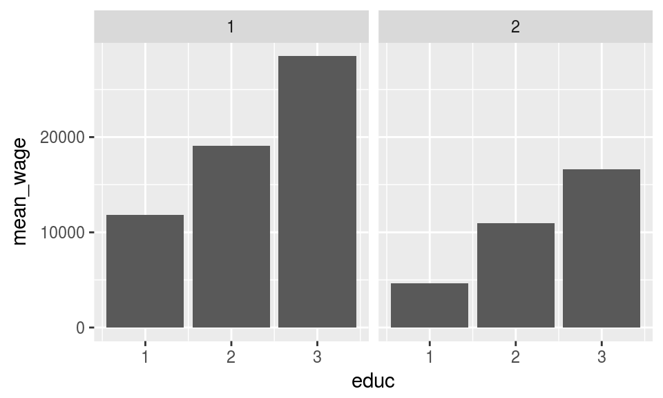
Then lets label the variables before plotting it with into.factor=FALSE

data_spss %>% 


  select(cname,sex,educ,pmi) %>% 


  na.omit() %>%


  group_by(cname,sex,educ) %>% 


  summarise(mean_wage = mean(pmi)) %>% 


  ungroup() %>% 


  mutate(sex = label_data(.,variable.data = "sex", metadata = meta_spss, into.factor=FALSE),
         educ = label_data(.,variable.data = "educ", metadata = meta_spss, into.factor=FALSE)) -> d_mean


ggplot(d_mean, aes(x=educ,y=mean_wage)) + geom_col() + facet_wrap(~sex)

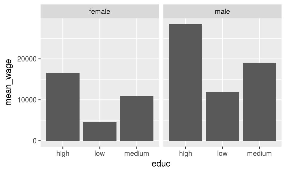
With into.factor set as FALSE the value labels are put in place as character ie. without any order. When set TRUE the value labels are forced into factors with same order of value labels as in the original SPSS/Stata files.

data_spss %>% 


  select(cname,sex,educ,pmi) %>% 


  na.omit() %>%


  group_by(cname,sex,educ) %>% 


  summarise(mean_wage = mean(pmi)) %>% 


  ungroup() %>% 


  mutate(sex = label_data(.,variable.data = "sex", metadata = meta_spss, into.factor=TRUE),
         educ = label_data(.,variable.data = "educ", metadata = meta_spss, into.factor=TRUE)) -> d_mean


ggplot(d_mean, aes(x=educ,y=mean_wage)) + geom_col() + facet_wrap(~sex)

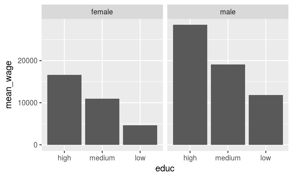
Package forcats is useful when you need to do more adjusting for the factors, for instance reversing the order of the factor labels as below.

data_spss %>% 


  select(cname,sex,educ,pmi) %>% 


  na.omit() %>%


  group_by(cname,sex,educ) %>% 


  summarise(mean_wage = mean(pmi)) %>% 


  ungroup() %>% 


  mutate(sex = label_data(.,variable.data = "sex", 
                          metadata = meta_spss, into.factor=TRUE),
         educ = label_data(.,variable.data = "educ", 
                           metadata = meta_spss, into.factor=TRUE)) %>% 


  mutate(
    sex  = forcats::fct_rev(sex),
    educ = forcats::fct_rev(educ)
  ) -> d_mean


ggplot(d_mean, aes(x=educ,y=mean_wage)) + geom_col() + facet_wrap(~sex)

Adding new variables

You often need to create new variables when working with social surveys, this is how you would do for age_class

First, lets make sure that variable ´age` is numeric with

meta_spss[meta_spss$code == "age",]$class == "numeric"

## [1] TRUE

then classify it into four categories

data_spss$age_class[data_spss$age < 20] <- 1

data_spss$age_class[data_spss$age >= 20 & data_spss$age < 40] <- 2

data_spss$age_class[data_spss$age >= 40 & data_spss$age < 60] <- 3

data_spss$age_class[data_spss$age >= 60] <- 4


as.data.frame(table(data_spss$age_class))

##   Var1 Freq
## 1    1  190
## 2    2  285
## 3    3  445
## 4    4  438

then lets add the new variable into metadata

new_row <- data_frame(
  code = "age_class",
  name = "age in four classes",
  value = 1:4,
  label = c("under 25",
            "25 to 39",
            "40 to 59",
            "60 or more"),
  class="factor"

)
meta_spss <- bind_rows(meta_spss,new_row)

Lets add the age class dimension to our analysis from above

data_spss %>% 


  select(cname,sex,educ,pmi,age_class) %>% 


  na.omit() %>%


  group_by(cname,sex,educ,age_class) %>% 


  summarise(mean_wage = mean(pmi)) %>% 


  ungroup() %>% 


  mutate(sex = label_data(.,variable.data = "sex", metadata = meta_spss, into.factor=TRUE),
         educ = label_data(.,variable.data = "educ", metadata = meta_spss, into.factor=TRUE),
         age_class = label_data(.,variable.data = "age_class", metadata = meta_spss, into.factor=TRUE)) -> d_mean


ggplot(d_mean, aes(x=educ,y=mean_wage)) + geom_col() + facet_grid(age_class~sex)

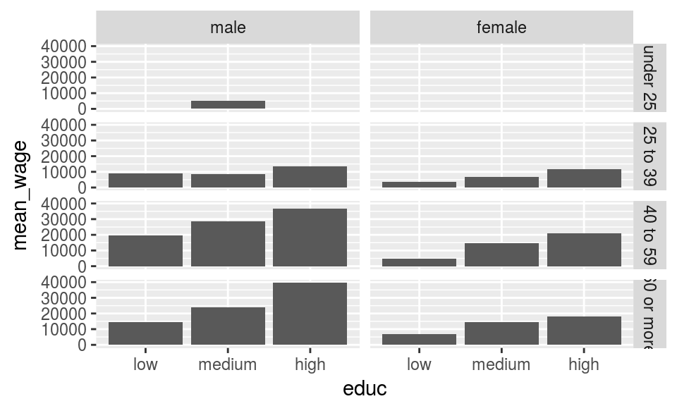
Again, this approach is very useful when working with shiny-applications as pointed out in this example at https://github.com/muuankarski/tidymetadata/tree/master/inst/shiny-examples/lisapp that can be lauched with tidymetadata::runExample()

Re-create the spss-data

You can then re-create spss-data from stripped data & meta-data using the function create_labelled_data() by passing the name of the raw data to data and matching tidy metadata to metadata

Add the variable labels ie. variable names or questions

d <- create_labelled_data(data = spss, metadata = meta_spss)

And this is how the first 15 variables look like with the attributes

str(d[1:15])

## Classes 'tbl_df', 'tbl' and 'data.frame':    1358 obs. of  15 variables:
##  $ hid     : atomic  1 1 2 2 2 2 3 4 4 4 ...
##   ..- attr(*, "label")= chr "unique unit identifier"
##   ..- attr(*, "format.spss")= chr "F9.0"
##   ..- attr(*, "display_width")= int 0
##  $ pid     : atomic  1 2 1 2 3 4 1 1 2 3 ...
##   ..- attr(*, "label")= chr "person identifier"
##   ..- attr(*, "format.spss")= chr "F8.0"
##   ..- attr(*, "display_width")= int 0
##  $ did     : atomic  198 198 198 198 198 198 198 198 198 198 ...
##   ..- attr(*, "label")= chr "unique country/year number"
##   ..- attr(*, "format.spss")= chr "F8.0"
##   ..- attr(*, "display_width")= int 0
##  $ dname   : atomic  it04 it04 it04 it04 ...
##   ..- attr(*, "label")= chr "country/year identifier"
##   ..- attr(*, "format.spss")= chr "A4"
##   ..- attr(*, "display_width")= int 0
##  $ cname   : atomic  Italy Italy Italy Italy ...
##   ..- attr(*, "label")= chr "country name"
##   ..- attr(*, "format.spss")= chr "A5"
##   ..- attr(*, "display_width")= int 0
##  $ iso2    : atomic  it it it it ...
##   ..- attr(*, "label")= chr "2-letter country abbreviation"
##   ..- attr(*, "format.spss")= chr "A2"
##   ..- attr(*, "display_width")= int 0
##  $ year    : atomic  2004 2004 2004 2004 2004 ...
##   ..- attr(*, "label")= chr "reference year"
##   ..- attr(*, "format.spss")= chr "F8.0"
##   ..- attr(*, "display_width")= int 0
##  $ wave    :Class 'labelled'  atomic [1:1358] 6 6 6 6 6 6 6 6 6 6 ...
##   .. ..- attr(*, "label")= chr "data wave"
##   .. ..- attr(*, "format.spss")= chr "F18.0"
##   .. ..- attr(*, "display_width")= int 0
##   .. ..- attr(*, "labels")= Named int [1:10] 0 1 2 3 4 5 6 7 8 9
##   .. .. ..- attr(*, "names")= chr [1:10] "Historical Wave" "Wave I" "Wave II" "Wave III" ...
##  $ pwgt    : atomic  3.7 3.7 8.9 8.9 8.9 ...
##   ..- attr(*, "label")= chr "person weight (normalised)"
##   ..- attr(*, "format.spss")= chr "F8.2"
##   ..- attr(*, "display_width")= int 0
##  $ ppopwgt : atomic  21820 21820 52526 52526 52526 ...
##   ..- attr(*, "label")= chr "person weight (inflated)"
##   ..- attr(*, "format.spss")= chr "F8.2"
##   ..- attr(*, "display_width")= int 0
##  $ pwgta   : atomic  NA NA NA NA NA NA NA NA NA NA ...
##   ..- attr(*, "label")= chr "additional person weight (for subsample)"
##   ..- attr(*, "format.spss")= chr "F8.0"
##   ..- attr(*, "display_width")= int 0
##  $ hhmem   :Class 'labelled'  atomic [1:1358] 1 1 1 1 1 1 1 1 1 1 ...
##   .. ..- attr(*, "label")= chr "household member (dummy)"
##   .. ..- attr(*, "format.spss")= chr "F23.0"
##   .. ..- attr(*, "display_width")= int 0
##   .. ..- attr(*, "labels")= Named int [1:2] 0 1
##   .. .. ..- attr(*, "names")= chr [1:2] "not household member" "household member"
##  $ relation:Class 'labelled'  atomic [1:1358] 1000 2000 1000 2000 3000 3000 1000 1000 2000 3000 ...
##   .. ..- attr(*, "label")= chr "relationship to household head"
##   .. ..- attr(*, "format.spss")= chr "F50.0"
##   .. ..- attr(*, "display_width")= int 0
##   .. ..- attr(*, "labels")= Named int [1:23] 1000 2000 2100 2200 3000 3100 3200 3300 4000 4100 ...
##   .. .. ..- attr(*, "names")= chr [1:23] "head" "spouse/partner" "spouse" "cohabiting partner" ...
##  $ partner :Class 'labelled'  atomic [1:1358] 110 110 110 110 200 200 200 110 110 200 ...
##   .. ..- attr(*, "label")= chr "partner"
##   .. ..- attr(*, "format.spss")= chr "F28.0"
##   .. ..- attr(*, "display_width")= int 0
##   .. ..- attr(*, "labels")= Named int [1:4] 100 110 120 200
##   .. .. ..- attr(*, "names")= chr [1:4] "has partner" "living with partner" "not living with partner" "does not have partner"
##  $ parents :Class 'labelled'  atomic [1:1358] NA NA NA NA 120 120 NA NA NA 120 ...
##   .. ..- attr(*, "label")= chr "living with parents"
##   .. ..- attr(*, "format.spss")= chr "F30.0"
##   .. ..- attr(*, "display_width")= int 0
##   .. ..- attr(*, "labels")= Named int [1:4] 100 110 120 200
##   .. .. ..- attr(*, "names")= chr [1:4] "living with parent(s)" "living with one parent" "living with two parents" "not living with parent(s)"

And you can then save it as .sav using haven

  haven::write_sav(d, path = "./lis_spss.sav")