plot of chunk smaterpolan02
SmarterPoland-package provides a straghtforward connection to Eurostat data. It is uninformatively described as:
A set of tools developed by the Foundation SmarterPoland.pl Tools for accessing and processing datasets presented on the blog SmarterPoland.pl.
But in real terms it has functionality only towards Eurostat. Here is a brief demo how you can search for material deprivation and then create a line plot at NUTS2 level.
library(SmarterPoland)## Loading required package: reshape
## Loading required package: plyr
##
## Attaching package: 'reshape'
##
## The following objects are masked from 'package:plyr':
##
## rename, round_any
##
## The following objects are masked from 'package:reshape2':
##
## colsplit, melt, recast
##
## Loading required package: rjsonsearchresults <- grepEurostatTOC("material deprivation")
df <- getEurostatRCV(kod = "ilc_mddd21")# time variable into numerical
df$time <- as.numeric(levels(df$time))[df$time]
cname <- subset(df, time == 2011)
# plot
library(ggplot2)
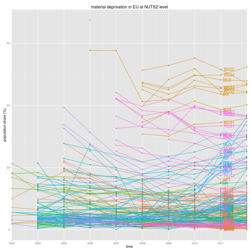
ggplot(df, aes(x=time,y=value, color=geo,group=geo)) +
geom_point() + geom_line() +
geom_text(data=cname,
aes(x=time,y=value,label=geo), hjust=-0.3) +
theme(legend.position="none") +
labs(title="material deprivation in EU at NUTS2-level",
y="population share (%)") +
coord_cartesian(xlim=c(2003,2012)) +
scale_x_continuous(breaks = 2003:2011)## Warning: Removed 854 rows containing missing values (geom_point).
## Warning: Removed 837 rows containing missing values (geom_path).
## Warning: Removed 14 rows containing missing values (geom_text).plot of chunk smaterpolan02
# subset geo-names only lenght of 2 characters
df$geo <- as.character(df$geo)
df$geo.n <- nchar(df$geo)
df <- subset(df, geo.n < 3)

cname <- subset(df, time == 2011)

# plot
library(ggplot2)
ggplot(df, aes(x=time,y=value, color=geo,group=geo)) +
  geom_point() + geom_line() +
  geom_text(data=cname,
            aes(x=time,y=value,label=geo), hjust=-0.3) +
  theme(legend.position="none") +
  labs(title="material deprivation in EU at NUTS2-level",
       y="population share (%)") +
  coord_cartesian(xlim=c(2003,2012)) +
  scale_x_continuous(breaks = 2003:2011)
## Warning: Removed 103 rows containing missing values (geom_point).
## Warning: Removed 93 rows containing missing values (geom_path).
## Warning: Removed 1 rows containing missing values (geom_text).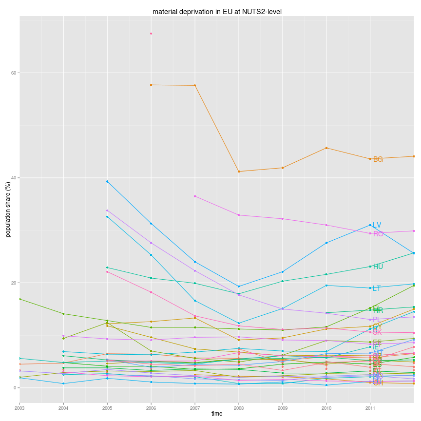
plot of chunk smaterpolan03
This is only a a brief description how to access and use spatial shapefiles of Europe published by EUROSTAT at Administrative units / Statistical units. Here I’m using the 1:60 million scale Shapefile from year 2010.
As a plotted data we use the nuts2-level rates of material deprivation which we imported from EUROSTAT on page SmarterPoland-package.
Same code as in SmarterPoland-package. excluding the plots.
library(SmarterPoland)
df <- getEurostatRaw(kod = "ilc_mddd21")
#
names(df) <- c("xx", 2011:2003)

df$unit <- lapply(strsplit(as.character(df$xx), ","), "[", 1)
df$geo.time <- lapply(strsplit(as.character(df$xx), ","), "[", 2)

df.l <- melt(data = df, id.vars = "geo.time", measure.vars = c("2003", "2004",
    "2005", "2006", "2007", "2008", "2009", "2010", "2011"))

df.l$geo.time <- unlist(df.l$geo.time) # unlist the geo.time variableSpatialPolygonDataFramedownload.file("http://epp.eurostat.ec.europa.eu/cache/GISCO/geodatafiles/NUTS_2010_60M_SH.zip",
destfile="NUTS_2010_60M_SH.zip")
# unzip to SpatialPolygonsDataFrame
unzip("NUTS_2010_60M_SH.zip")
library(rgdal)## rgdal: version: 0.8-16, (SVN revision 498)
## Geospatial Data Abstraction Library extensions to R successfully loaded
## Loaded GDAL runtime: GDAL 1.7.3, released 2010/11/10
## Path to GDAL shared files: /usr/share/gdal/1.7
## GDAL does not use iconv for recoding strings.
## Loaded PROJ.4 runtime: Rel. 4.7.1, 23 September 2009, [PJ_VERSION: 470]
## Path to PROJ.4 shared files: (autodetected)map <- readOGR(dsn = "./NUTS_2010_60M_SH/data", layer = "NUTS_RG_60M_2010")## OGR data source with driver: ESRI Shapefile
## Source: "./NUTS_2010_60M_SH/data", layer: "NUTS_RG_60M_2010"
## with 1920 features and 4 fields
## Feature type: wkbPolygon with 2 dimensions# as the data is at NUTS2-level, we subset the spatialpolygondataframe
map_nuts2 <- subset(map, STAT_LEVL_ <= 2)
# dim show how many regions are in the spatialpolygondataframe
dim(map_nuts2)## [1] 467 4# dim show how many regions are in the data.frame
dim(df)## [1] 208 14# Spatial dataframe has 467 rows and attribute data 223.
# We need to make attribute data to have similar number of rows
NUTS_ID <- as.character(map_nuts2$NUTS_ID)
VarX <- rep("empty", 467)
dat <- data.frame(NUTS_ID,VarX)
# then we shall merge this with Eurostat data.frame
dat2 <- merge(dat,df,by.x="NUTS_ID",by.y="geo.time", all.x=TRUE)
## merge this manipulated attribute data with the spatialpolygondataframe
# there are still duplicates in the data, remove them
dat2$dup <- duplicated(dat2$NUTS_ID)
dat3 <- subset(dat2, dup == FALSE)
## rownames
row.names(dat3) <- dat3$NUTS_ID
row.names(map_nuts2) <- as.character(map_nuts2$NUTS_ID)
## order data
dat3 <- dat3[order(row.names(dat3)), ]
map_nuts2 <- map_nuts2[order(row.names(map_nuts2)), ]
## join
library(maptools)
shape <- spCbind(map_nuts2, dat3)## fortify spatialpolygondataframe into data.frame
library(ggplot2)
library(rgeos)
shape$id <- rownames(shape@data)
map.points <- fortify(shape, region = "id")
map.df <- merge(map.points, shape, by = "id")
# As we want to plot map faceted by years from 2003 to 2011
# we have to melt it into long format
library(reshape2)
map.df.l <- melt(data = map.df, id.vars = c("id","long","lat","group"),
measure.vars = c("X2003", "X2004",
"X2005", "X2006",
"X2007", "X2008",
"X2009", "X2010", "X2011"))
# year variable (variable) is class string and type X20xx.
# Lets remove the X and convert it to numerical
library(stringr)
map.df.l$variable <- str_replace_all(map.df.l$variable, "X","")
map.df.l$variable <- factor(map.df.l$variable)
map.df.l$variable <- as.numeric(levels(map.df.l$variable))[map.df.l$variable]Map shows proportion of materially deprived households at the NUTS2 level. Grey color indicates missing data.
library(ggplot2)
# plot faceted by year
ggplot(map.df.l, aes(long,lat,group=group)) +
  geom_polygon(aes(fill = value)) +
  geom_polygon(data = map.df.l, aes(long,lat),
               fill=NA,
               color = "white",
               size=0.1) + # white borders
  coord_map(project="orthographic", xlim=c(-22,34),
              ylim=c(35,70)) + # projection
  facet_wrap(~variable, ncol=2) +
  theme_minimal()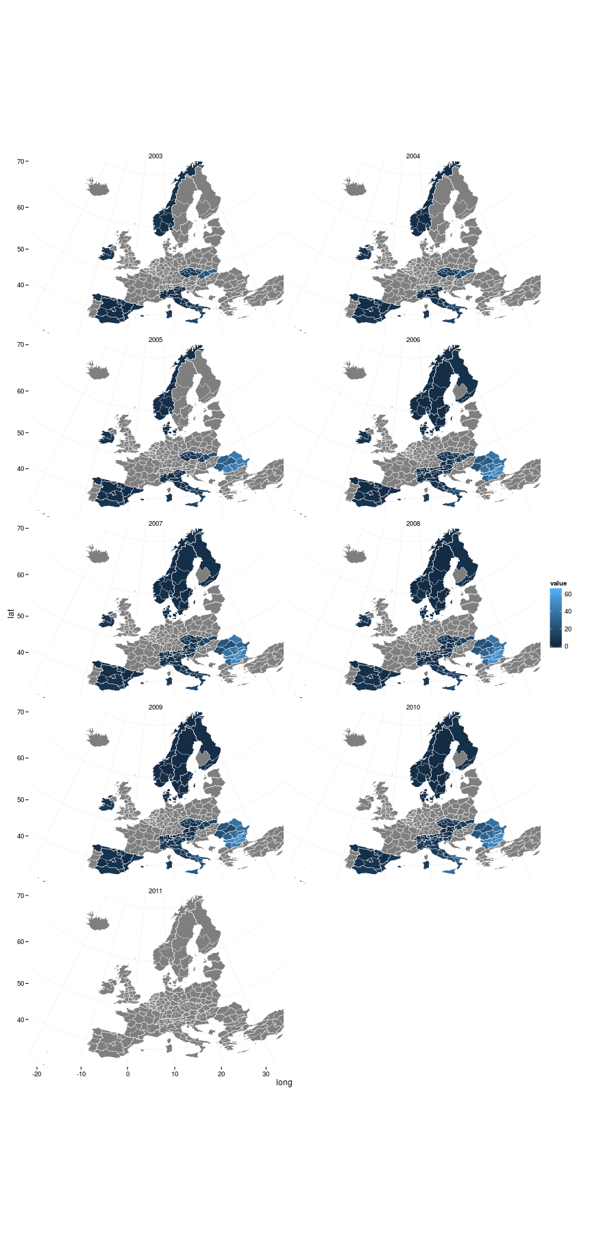
plot of chunk smaterpoland4